Benchmark Before You Refactor: A Latency Harness for HFT C++ Systems

Table of Contents

• The Refactor Nobody Could Argue About
• Why the Average Lies: Coordinated Omission and the Tail
• What My Own “100 Microseconds” Line Is Missing
• Baseline First: What “Measure the Old Code” Actually Requires
• Measuring on a Machine That Is Lying to You
• What LLVM, Rust, ClickHouse, Chromium, and Go Do About Regressions
• What a Merge Gate Does Not Guarantee
• The Harness: Seven Rows That Make Two Numbers Comparable
• What It Costs to Build, and What to Build First
• Put the Harness in Before the First Merge

The Refactor Nobody Could Argue About

Years ago, I met with a team of 8 engineers, deep in C++, and their architecture was still a disaster.

Small proprietary trading firm, high frequency. The engineers were very good and very experienced, already working pretty well.

They had Python and C++ mixed together, with independent systems and processes scattered around the whole organization. For obvious reasons, the C++ processes were put in the sensitive/hot path.

My read was that parts of it needed a big refactor. Before starting any of that, I sat with their CTO and we built the benchmark.

We measured the old systems and subsystems first, on the code they already had, so that afterwards we could say what a change had done.

Then it became a loop. Measure, improve those processes, measure again, until they hit the latencies they were after.

Thank you for reading this post, don't forget to subscribe!

Subscribe by Email

We reached under 100 microseconds back then, software only. We knew we could go lower, and stopped there, because for what they were doing it was enough.

The key was to give them the right framework, so they could keep benchmarking everything they changed or added.

Even if it sounds obvious, when refactoring, wire the benchmark into the change process before you start, so every merge re-runs it and an improvement cannot silently regress.

That is the post as I published it on LinkedIn. One line in it deserves a closer look before anything else: “for obvious reasons, the C++ processes were put in the sensitive/hot path.” C++ gives a hot path manual, deterministic memory management, no interpreter dispatch sitting between a line of code and the instruction that runs it, no single global lock serializing execution the way Python’s own interpreter lock does, and tighter control over allocation and cache locality than most managed runtimes hand you by default. It also never pauses the whole process to reclaim memory on its own schedule. Discord’s Read States service, running on Go, took latency spikes roughly every two minutes, traced directly to the minimum interval at which Go’s runtime forces a garbage collection pass regardless of memory pressure. Discord’s own account describes the result as higher 99th percentile latency times. C++ is the common choice for a hot path built this way, though never the only one. Rust delivers the same absence of a garbage collector with memory safety C++ does not provide, and in practice some desks run tuned Java or C# on parts of the hot path too, with results that depend heavily on what the runtime’s own JIT and garbage collector are doing underneath.

The rest of that post is the actual subject of this article, and the architecture is not it. Before touching a line of the system, the CTO and I built a way to measure it. That decision, more than the eventual latency number, is what made the case for changing anything arguable instead of opinion driven. Convincing a room of eight very good, very experienced engineers to rip out infrastructure they built and already trust is a persuasion problem before it is a technical one, and the only durable way to win it is to make the current state and the proposed state both checkable, before either one is treated as settled.

Everything below sets out what that checking requires, including one honest look at my own sentence above.

Why the Average Lies: Coordinated Omission and the Tail

A benchmark that reports a single average throws away the part of a latency distribution that matters operationally: the tail. This is a specific, well-documented measurement bug with a name of its own: coordinated omission.

The bug shows up whenever a load generator waits for a response before it issues its next request. Gil Tene’s wrk2, an HTTP load-testing tool built specifically to correct it, states the mechanism directly. A closed-loop generator “exhibits a strong Coordinated Omission effect, through which most of the high latency artifacts exhibited by the measured server will be ignored,” because “high latency responses result in the load generator coordinating with the server to avoid measurement during high latency periods.” In plain terms, if a test harness only sends its next unit of work after the last one returns, the one moment the system under test stalls is the exact moment the harness stops sampling it. The stall vanishes from the results because the tool that would have caught it was busy waiting.

wrk2‘s fix is to stop timing a request from when it was actually sent, and instead time it from when it should have been sent, on a fixed, constant-throughput schedule. Load keeps arriving on that schedule whether the system under test is keeping up or not, the same way market data keeps arriving whether a feed handler is keeping up or not.

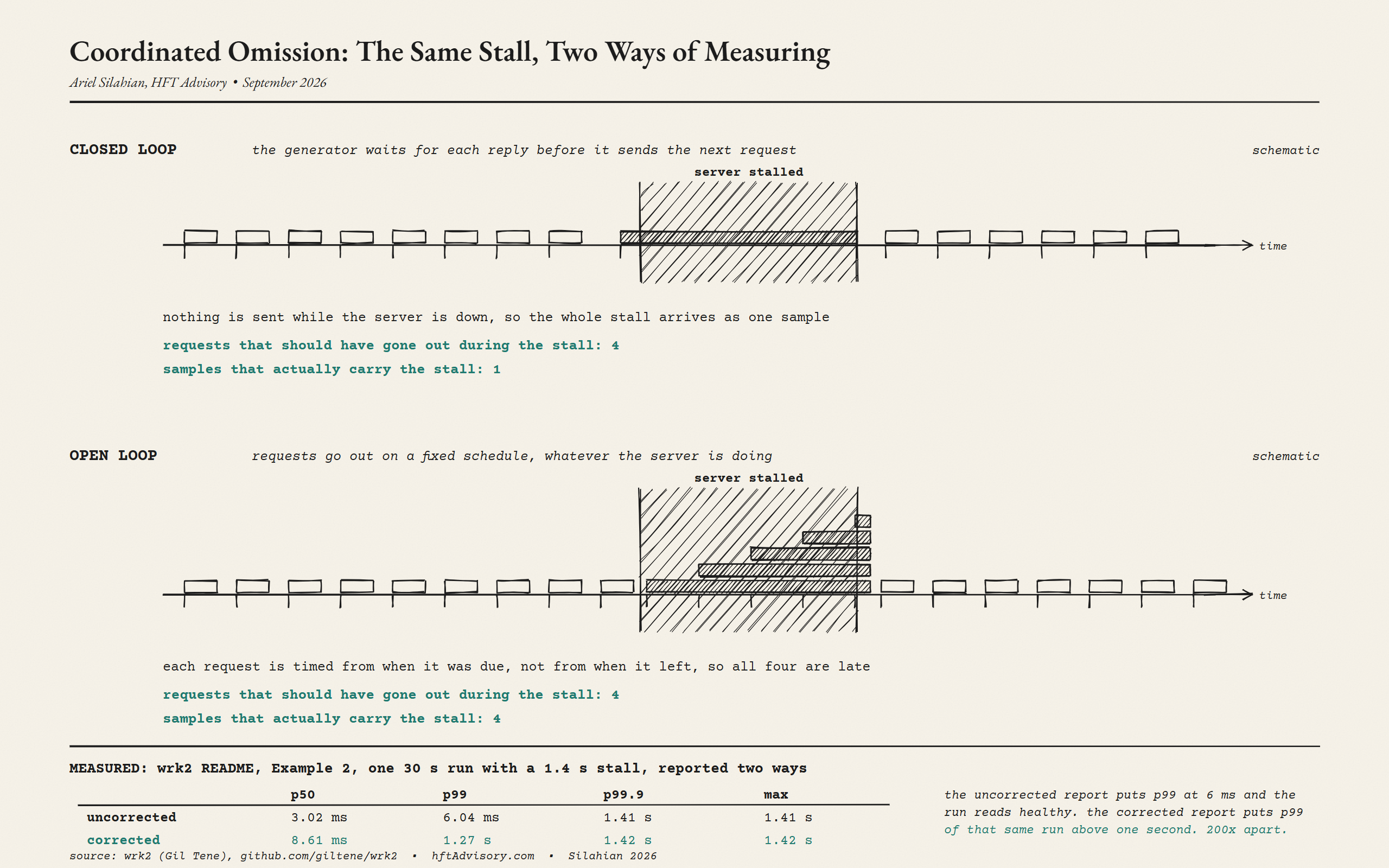
The correction is not a rounding adjustment. In wrk2‘s own demonstration, a single 1.4-second stall was introduced into an otherwise healthy web server, and the same 30-second run was then reported two ways. The traditional, coordinated-omission-susceptible report: median 3.02 milliseconds, 99th percentile 6.04 milliseconds, 99.9th percentile 1.41 seconds. The corrected report, on the identical run: median 8.61 milliseconds, 99th percentile 1.27 seconds, 99.9th percentile 1.42 seconds. Gil Tene’s own summary of that gap is a corrected report “reporting a 99%’ile that is 200x (!!!) larger than that of the traditional measurement technique that was susceptible to Coordinated Omission.” Read the uncorrected column on its own and the run looks healthy, with a 99th percentile of 6 milliseconds. The corrected column says the 99th percentile of that same run was over a second.

Acting on this does not require expensive tooling. HdrHistogram, the histogram library wrk2 uses internally through Mike Barker’s C port, documents value recording times as low as three to six nanoseconds on the Intel CPUs its own implementation was benchmarked on, with a constant memory footprint regardless of sample count and no allocation on the recording path. Treat that as a floor measured on one port rather than a guarantee for yours, and the conclusion still holds: keeping the full distribution is cheap enough that discarding one down to a mean is not an engineering tradeoff.

What My Own “100 Microseconds” Line Is Missing

I want to hold my own sentence from the post above to the same standard: “we reached under 100 microseconds back then, software only.” Read it the way you would read a vendor’s benchmark slide, and it fails the test the section above just laid out. It never says which two points in the system the number was measured between, which statistic it reports (a mean, a median, a 99th percentile, a maximum), or what load the system was under when it was captured, closed-loop or open-loop, idle or under a synthetic burst or under replayed market data. And “software only” is carrying weight without defining its own edge. Does the span start at the network card handing a packet to the kernel, or at the first line of application code already holding that packet in a buffer? Those are two different starting lines, and on a real network stack the distance between them is not zero.

What I stand behind is what the sentence was about. The number came off the harness we had just built, measured against a baseline taken from the same code before we changed it, with no hardware acceleration anywhere in the path. What I will not do is reconstruct the span and the percentile from memory and present them as fact, because a latency number assembled after the event is the thing this article exists to argue against.

So take the shape rather than the number. Any latency figure worth putting in front of someone else carries four things: the two timestamps it sits between and the clock each one came from, the statistic it reports (p50, p99, p99.9 or max, never “average”), the load model that produced it, and what was excluded from the path. “Under 100 microseconds, software only” carries none of them. A number that carries all four reads like this: p99.9, NIC receive to NIC transmit, PTP-disciplined hardware timestamps at both ends, under an open-loop replay of a recorded peak-hour session, no hardware acceleration in the path. The second version is something a reader can argue with. The first is a boast.

Baseline First: What “Measure the Old Code” Actually Requires

“We measured the old systems and subsystems first, on the code they already had, so that afterwards we could say what a change had done.” That line describes a before-and-after comparison, and a before-and-after comparison only tells you what a change did if everything except the change stayed fixed. That sounds obvious. In practice it is routinely not what happens.

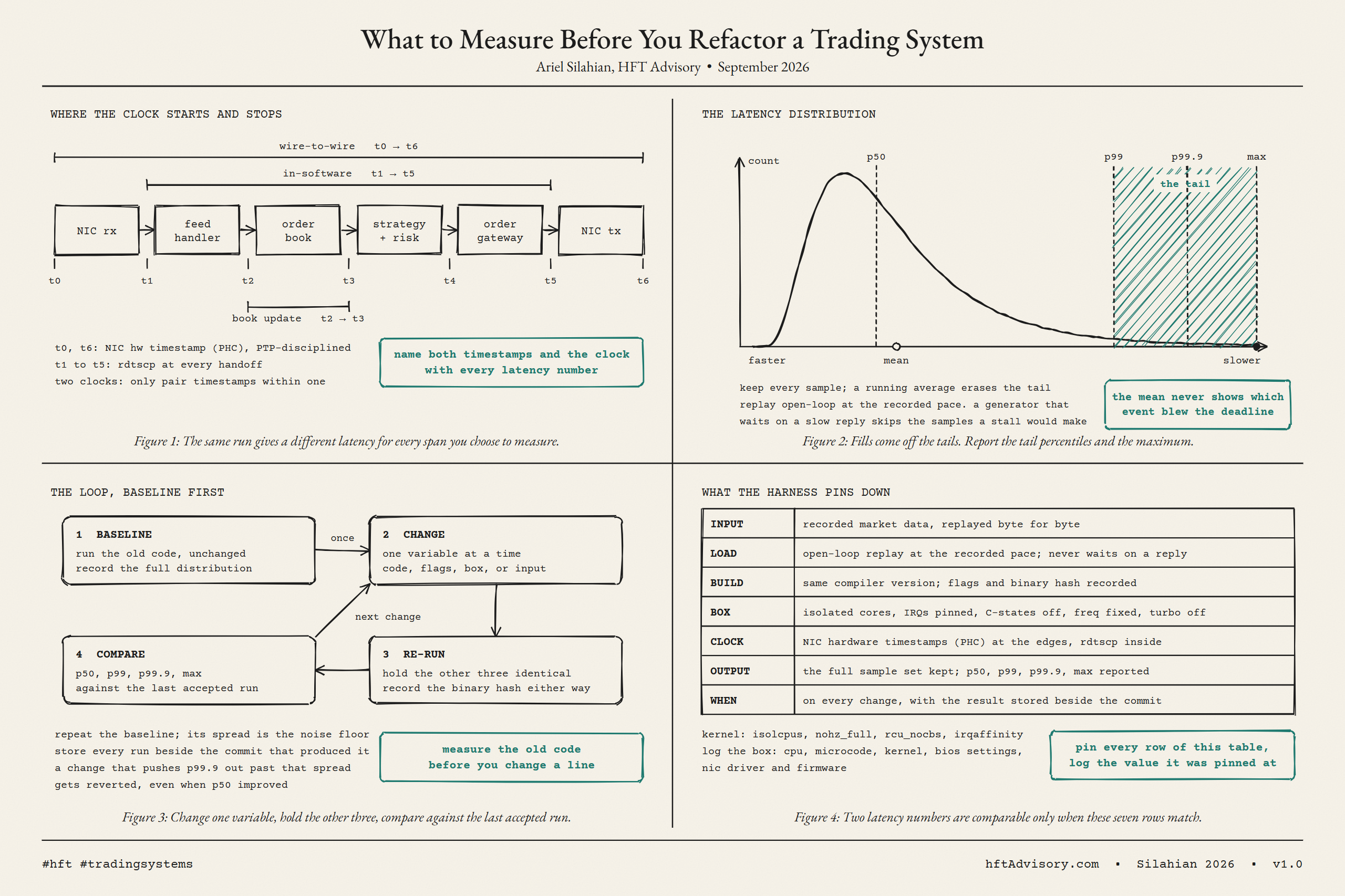
The loop the post describes, measure, improve, measure again, is a sequence in time: run the baseline once, then repeatedly change one thing, re-run, and compare the new result against the last accepted result rather than the original baseline. Repeating the baseline itself, unchanged, on its own, matters more than it sounds like it should. Its spread across repeated runs is the noise floor: the amount of variation the system produces with nothing changed at all. A later result that lands inside that spread has told you nothing. A result that pushes the 99.9th percentile outside that spread, even while the median improved, is a regression, and gets reverted regardless of what the average said.

That loop only produces a trustworthy answer if “measured” means the same thing on both sides of it. In practice, seven things have to stay fixed between a baseline run and the comparison run measured against it: what data went in, how that data was fed in, which compiler produced the binary and with which flags, what physical machine and configuration it ran on, which clock produced the timestamps, what got recorded out of the run, and how often the whole comparison gets repeated. The code is the one variable the loop exists to test. Let any of those seven drift while the code changes, and the result no longer tells you which of them produced what you are looking at. The full version of that list, and exactly what each row pins down, is the harness later in this piece.

One more line from the post is the one I trust least as a settled fact: “the key was to give them the right framework, so they could keep benchmarking everything they changed or added.” That is my read on why the engagement held up after I left. I have no controlled comparison to point to against a team that got the same refactor without the harness. What I have is a pattern I would bet on again: a team that owns its own measurement tends to keep using it once the outside advisor is gone, and a team handed a one-time report mostly does not.

Measuring on a Machine That Is Lying to You

Two runs on “the same machine” are often not comparable, because the machine itself is not holding still, starting with the clock timing it.

Clock read granularity is a confound on its own, and it is platform-dependent in a way that will quietly invalidate a sub-microsecond comparison. Aleksey Shipilev measured nanosecond timer granularity across platforms in Nanotrusting the Nanotime and reported roughly 26.3 nanoseconds on Linux against roughly 371.4 nanoseconds on Windows 7, for what is nominally the same kind of call. That block of his results prints its decimals with commas, and his own reading of the Windows figure is about 370 nanoseconds of precision, which means 26 consecutive calls can return the same value before the 27th moves. The call itself stays cheap on both platforms. What changes, by a factor of fourteen, is how finely it resolves, and a timer that cannot resolve the effect you are chasing will report it as zero. Whatever the exact figure is on your own operating system and hardware today, that is the class of confound this row of the harness exists to close off: measure it, do not assume it away.

The clock can drift against itself too, even on a single box. The Linux kernel documents that the x86 timestamp counter can drift sched_clock() between CPUs on the same machine, which is why the kernel ships CONFIG_HAVE_UNSTABLE_SCHED_CLOCK as a workaround. A software timer read inside one process is a per-CPU value unless proven otherwise. For anything crossing a real boundary, the network card itself, Linux exposes hardware packet timestamping through the SO_TIMESTAMPING socket option, including SOF_TIMESTAMPING_RAW_HARDWARE, and the PTP Hardware Clock is the kernel’s abstraction for the NIC-resident hardware clock used for IEEE-1588 time synchronization. Wire-side timestamps from a disciplined hardware clock and in-process timestamps from a CPU counter are two different clocks. Pairing a value from one against a value from the other and calling the difference a duration means comparing two clocks that were never proven to agree with each other.

Below the clock, the operating system itself absorbs jitter a benchmark can pick up without it ever showing as “the code got slower.” The kernel’s isolcpus parameter isolates a named set of CPUs from the scheduler’s ordinary load balancing. nohz_full stops the periodic scheduling tick on those cores and, in the same step, offloads their RCU callbacks the way rcu_nocbs does explicitly, which the kernel documentation credits with reducing OS jitter, “useful for HPC and real-time workloads.” IRQ affinity, set through /proc/irq/IRQ#/smp_affinity, decides which core services a given hardware interrupt, and an interrupt landing on your benchmark’s core mid-run reads, in the result, exactly like your code getting slower. The intel_idle driver’s max_cstate caps how deep an idle CPU is allowed to sleep before a request wakes it back up, and intel_pstate exposes a no_turbo setting to hold frequency fixed instead of letting it climb and fall with thermal and power headroom. Huge pages, tracked through /proc/sys/vm/nr_hugepages, change how address translation gets paid for, and are worth pinning to an explicit value rather than leaving to whatever the box happened to be configured with that day.

ClickHouse has an open RFC to rewrite its performance comparison tests that names two of these as the fix: set the CPU governor to performance mode, which disables frequency scaling, and disable turbo boost, which the RFC calls “the single biggest source of thermal-dependent variance.” The same document records their current setup as no CPU governor pinning, no turbo boost control, and no other OS-level tuning, and lists the variance that follows among the problems it is trying to solve. A team running one of the more scrutinized open-source performance pipelines in the industry has not turned these off yet, and treats that as a known weakness in its own numbers. Worth taking as a default for any benchmark, including yours.

What LLVM, Rust, ClickHouse, Chromium, and Go Do About Regressions

None of this is unique to trading systems. The five projects below all run some version of continuous, gated measurement, and the shape of it repeats across languages and organizations that otherwise have nothing to do with each other.

LLVM has run LNT, its own performance-tracking software, for years, built for two stated use cases: “post-commit detection of performance regressions and improvements” and “pre-commit analysis of the impact of a patch on performance.” The Rust compiler team runs a standing triage against its own benchmark suite: “we regularly triage the effects of merged PRs on rustc’s speed and memory usage.” That process caught a real regression on 2025-11-03. A routine dependency bump to cc-rs regressed instruction counts by a mean of 0.7 percent, ranging from 0.3 to 3.7 percent across 259 benchmarks. The triage recorded the likely cause, in its own words perhaps, as the update no longer passing a -flto flag to jemalloc, and the change was reverted. The revert measured a mean improvement of 0.7 percent, ranging from negative 3.6 to negative 0.3 percent, across 251 benchmarks. It was caught only because the harness re-ran on every merge instead of waiting for a complaint.

ClickHouse found a roughly 18 percent regression in its own SSB benchmark’s queries-per-second between two commits, traced it to lock contention created by a per-query profiler-timer syscall, fixed it with a per-thread timer id instead, and measured the recovery at 17.7 percent. Chrome runs “multiple performance labs in which benchmarks are run on continuous builds to pinpoint performance regressions down to individual changelists,” staffed by rotating performance sheriffs, backed by an automated bisection service named Pinpoint that narrows a regression to the specific commit responsible. The Go project states its comparison policy without hedging: “we never report performance numbers in isolation, and only relative to some baseline,” because “comparing performance data taken far apart in time, even on the same hardware, can result in a lot of noise.”

Across five projects and three languages the premise is the same. A performance number is not evidence of anything until a baseline sits next to it, measured close in time, on the same machine, gated on every change instead of checked occasionally when someone complains.

What a Merge Gate Does Not Guarantee

The post above ends with a specific claim: “wire the benchmark into the change process before you start, so every merge re-runs it and an improvement cannot silently regress.” I want to hold that sentence to the same standard I held my own latency number to earlier in this piece, because stated flatly it promises more than a gate can deliver.

What a merge gate converts is “nobody looked” into “something looked, every time.” That is a useful change on its own. The clearest evidence for its limit comes from the most demanding test bed available: Chromium’s own continuous integration. Haben, Habchi, Papadakis, Cordy and Le Traon measured a state-of-the-art flakiness-prediction model against real Chromium CI data in The Importance of Discerning Flaky from Fault-triggering Test Failures and found that even at 99.2 percent precision on the alerts it did fire, the model still missed approximately 76.2 percent of all regression faults in that process. High precision on what a gate does flag says nothing about how much of the total regression traffic it covers, and on real production CI that gap runs large.

A gate can also fail the other way, by crying wolf until nobody trusts it. ClickHouse names the mechanism plainly in the problems list of that same RFC: “a query that historically fluctuates by 15% will never catch an 8% regression, even if that regression is real and consistent.” Daniel Marbach, writing on performance regression testing without fooling yourself, reports build-to-build variance on the identical unchanged revision running from 1.5 to 2 seconds in a clean environment up to 12 to 36 seconds on noisy shared hardware, and reaches the conclusion I would put the same way: “a flaky performance gate is worse than no gate,” because “if people stop trusting the signal, the tooling has already lost.” His practical fix, prune down to a handful of investigation benchmarks kept for debugging and a smaller set of hot-path benchmarks kept as merge gates, is the right instinct.

That still leaves the question none of the sources answers for you: which benchmarks earn the right to block a merge. The rule I use follows from the ClickHouse number above. Measure a benchmark’s own noise floor first, by repeating the baseline against itself on the box you will gate from, and let it block a merge only if that floor is narrower than the smallest regression you would genuinely revert for. A benchmark whose own spread is 15 percent cannot police an 8 percent regression; gating on it buys alerts and no information. Keep that one for investigation and let something quieter hold the gate. That is my inference from the numbers above rather than a finding any of these sources states, and it is falsifiable in an afternoon: if the suite currently blocking your merges has a wider noise floor than your revert threshold, it is already lying to you.

There is a methodological case for gating narrow microbenchmarks specifically. Japke, Witzko, Grambow and Bermbach injected three known performance defects into a controlled study presented at UCC 2023 and found that microbenchmarks detected all three earlier than application-level benchmarks did, in some cases at the lowest severity level tested, while the application-level benchmarks “raised false positive alarms, wrongly detected performance improvements, and detected the performance issues later.” That is an advantage for the kind of narrow, hot-path microbenchmark this harness is built around, and it is only part of the picture. Google’s own performance engineering team describes production testing as a four-tier hierarchy, microbenchmark, single-task loadtest, cluster loadtest, production, and states outright that “it is not uncommon for the first and last to disagree.” A number from a gate is not a verdict on its own. Vyacheslav Egorov, who describes himself on his own site as a compiler engineer, put it this way about benchmark results generally: “benchmarks are not numerology. Their results are not a divine revelation. Benchmarks are experiments. Their results are meaningless without interpretation and validation.”

So that closing line promises less than it reads. A gate wired into the merge process guarantees that something looked. It does not guarantee that the something found the regression. Those are two different promises, and only one of them is one I can keep on every merge.

The Harness: Seven Rows That Make Two Numbers Comparable

This is the practical version of everything above, reduced to the checklist I use. Two latency numbers, whether they are two runs of the same system a week apart or an old architecture measured against a proposed rewrite, are comparable only when all seven of these rows match.

Row	What it pins down
INPUT	Recorded market data, replayed byte for byte
LOAD	Open-loop replay at the recorded pace; never waits on a reply
BUILD	Same compiler version; flags and binary hash recorded
BOX	Isolated cores, IRQs pinned, C-states off, frequency fixed, turbo off
CLOCK	NIC hardware timestamps (PHC) at the edges, a monotonic hardware counter inside
OUTPUT	The full sample set kept; p50, p99, p99.9, max reported
WHEN	On every change, with the result stored beside the commit

LOAD is the row that ties directly back to coordinated omission. Recorded market data replayed open-loop, at the pace it originally arrived, never pauses to wait for your system’s reply the way a closed-loop generator does. A stall in your code shows up in the samples instead of quietly disappearing from them.

CLOCK resolves the two-clock problem from earlier instead of just describing it. At the two edges of the system, where a packet arrives from the wire and where a response leaves back onto it, the timestamp comes from the NIC’s own hardware clock, PTP-disciplined. Inside the system, at every handoff between components, the timestamp comes from a monotonic hardware counter read at that handoff. The rule that makes both usable together is simple and does not bend: pair timestamps only when they came from the same clock. A wire-to-wire duration needs both of its ends from the hardware clock. An in-software duration needs both of its ends from the same counter.

Naming the clock is also what closes the gap in my own “software only” line from earlier. On a run built to this harness, that span has an actual name: wire-to-wire runs from the NIC receiving a packet to the NIC transmitting the response, in-software runs from the point the feed handler first touches the packet to the point the order gateway hands the response back to the wire, and a book update specifically is the narrower span from the order book receiving the event to the strategy and risk layer acting on it. Reporting a latency number without saying which of those three it names is the gap this whole article has been arguing against, my own line from the top of this piece included.

BOX means logging more than “same server.” It means the same CPU, the same microcode revision, the same kernel build, the same BIOS power and frequency settings, and the same NIC driver and firmware version, recorded alongside the result instead of assumed. BUILD means the same compiler version with the flags and the resulting binary’s hash both recorded, because the cc-rs regression two sections ago cost 0.7 percent from a silently dropped -flto flag.

None of this needs custom tooling to implement. C++ teams have Google Benchmark, which requires C++17, and nanobench, a header-only library that reports nanoseconds per operation, instructions per operation, cycles per operation, IPC, and branch-miss percentage directly, and whose own documentation claims roughly an 80x lower overhead for the harness itself than Google Benchmark. On the JVM the answer is JMH, the benchmark harness built into the OpenJDK project, and in Rust it is Criterion.rs, a statistics-driven microbenchmarking library. The tooling to record OUTPUT correctly, a full sample set instead of a mean, already exists in whichever language you are running. The discipline is in wiring it to the other six rows.

The fourth step of the baseline-first loop, COMPARE, is where WHEN and OUTPUT meet. Repeat the baseline before comparing anything against it. Its own spread across repeats is the noise floor. That number is specific to your own box, your own workload, and how well the other six rows are held fixed. A change that widens the tail while improving the median still increases how often a single fill lands far from the rest of the run. Reverting on the 99.9th percentile, even when the median improved, is the correct call on a hot path.

What It Costs to Build, and What to Build First

I build these seven rows in the order below, never all at once. They are not equally expensive, and they do not pay off in the order the table lists them.

Start with INPUT and OUTPUT. A recorded session you can replay byte for byte, and a harness that keeps every sample instead of a mean, are the two rows that make every later row worth having. Without them there is nothing to compare and nothing to compare it against. A team that already captures raw market data has most of INPUT already, and OUTPUT is a library call. That is the cheap half of the harness.

Then LOAD, because it is the row that changes the answer rather than the precision. Replaying at the recorded pace instead of as fast as the system will accept is usually a change to a few lines of the replay driver, and it is the difference between a harness that shows stalls and one that hides them.

BOX comes next and is where the calendar time goes. Pinning cores, fixing frequency, turning off turbo and the deeper idle states, and then recording all of it beside the result, is not difficult work, but it touches machine provisioning and it needs someone with root on the box you are going to gate from. On a small team this is the row that waits on somebody else.

CLOCK and BUILD are cheap once the rest exists. They need a monotonic counter at every handoff, hardware timestamps at the edges if the hardware supports it, and the compiler version, flags and binary hash written next to the result. WHEN, the row that puts the harness in the merge path, is last on purpose: gating on a benchmark whose noise floor you have not measured is the failure mode two sections ago describes.

A team of three can have INPUT, OUTPUT and LOAD running against their own hot path in days rather than sprints, and that partial harness is already enough to make a refactor argument. The full seven rows is a longer piece of work, and most of that length is BOX and the discipline of keeping the log; writing the code is the smaller share.

Put the Harness in Before the First Merge

Here is a test you can run on your own last refactor, right now, without waiting for the next one. Find the commit or the pull request that claimed a performance win. Check it against the seven rows above: was the input identical and replayed the same way, on the same build, on the same box, timed off the same clock, with the full distribution kept, and repeated more than once. If any one of those seven did not match between the before and the after, the claimed win is not proven yet. It is asserted, and an assertion is exactly what a benchmark exists to replace.

I do not have a clean answer for how wide a noise floor is too wide to trust the gate built on top of it. ClickHouse’s own team names 15 percent as a fluctuation their randomized test cannot reliably separate from a real, consistent 8 percent regression, on their workload, on their hardware. I have not measured that threshold for a FIX decoder or an order book, and I am not going to invent one here. I rely on the loop instead: measure the old code before changing a line, repeat that baseline until its own spread is known, and only then start changing one thing at a time.

If you want a second pair of eyes on which of these seven rows your last comparison held constant, that is the kind of review I do. I read the harness, then the last few performance claims that came out of it, and say which of them the evidence actually supports. hftAdvisory.com is where that starts.

---

This article was originally shared as a LinkedIn post.