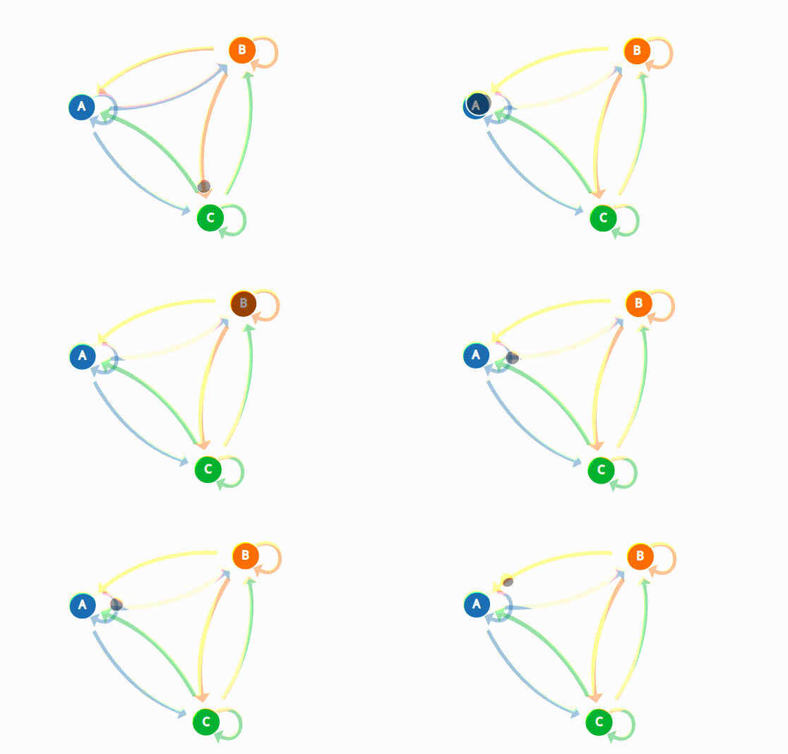
This article was originally posted by Nagesh Singh Chauhan and you can read it here.
The article contains a brief introduction to Markov models specifically Markov chains with some real-life examples.

Thank you for reading this post, don't forget to subscribe!
The Weak Law of Large Numbers states:
“When you collect independent samples, as the number of samples gets bigger, the mean of those samples converges to the true mean of the population.”
Andrei Markov didn’t agree with this law and he created a way to describe how random, also called stochastic, systems or processes evolve over time.
Markov believed independence was not a required condition for the mean to converge. So he set out to define how the average of the outcomes from a process including dependent random variables could converge over time.
The system is modeled as a sequence of states and, as time goes by, it moves in-between states with a specific probability. Since the states are connected, they form a chain.
Markov model
A Markov model(process) is a Stochastic process for randomly changing systems where it is believed that future states do not depend on past states. These models show all possible states as well as the transitions, rate of transitions, and probabilities between them.
Markov models are frequently used to model the probabilities of various states and the rates of transitions among them. The method is generally used to model systems. Markov models can also be used to identify patterns, make predictions, and learn the statistics of sequential data.
A Markov process is a process that is capable of being in more than one state, can make transitions among those states, and in which the states available and transition probabilities depend only upon what state the system is currently in. In other words, there is no memory in a Markov process.
There are four types of Markov models that are used situationally:
- Markov chain – used by systems that are autonomous and have fully observable states
- Hidden Markov model – used by systems that are autonomous where the state is partially observable.
- Markov decision processes – used by controlled systems with a fully observable state.
- Partially observable Markov decision processes – used by controlled systems where the state is partially observable.

Markov models can be manifested in equations or in graphical models. Graphic Markov models typically use circles (each containing states) and directional arrows to show potential transitional changes between them. The directional arrows are labeled with the rate or the variable one for the rate. Applications of Markov modeling include modeling languages, natural language processing (NLP), image processing, bioinformatics, speech recognition, and modeling computer hardware and software systems.
Markov chain
Markov chain is the purest Markov model.
The algorithm known as PageRank, which was originally proposed for the internet search engine Google, is based on a Markov process.
Reddit’s Subreddit Simulator is a fully-automated subreddit that generates random submissions and comments using markov chains, so cool!
Markov chains, named after Andrey Markov, are mathematical systems that jump from one “state” (a situation or set of values) to another. For example, if you do a Markov chain model of a baby’s routine, you might add “playing,” “eating”, “sleeping,” and “crying” as states, which together with other routines could form a ‘state space’: a list of all possible states. In addition, on top of the state space, a Markov chain represents the probability of hopping, or “transitioning,” from one state to any other state—e.g., the chance that a baby currently playing will fall asleep in the next five minutes without crying first.

The above diagram depicting a two-state Markov chain, with the states, labeled E and A. Each number depicts the probability of the Markov process changing from one state to another state, with the direction indicated by the arrow. For example, if the Markov process is in state A, then the probability it changes to state E is 0.4, while the probability it remains in state A is 0.6.

In Markov Chain, the next stage of the process depends only on the previous state and not on the prior sequence of events. Let us think about a stochastic process {Xn}, n=0,1,2,3,4 .. which has a discrete State Space S and satisfies the Markov Property. This is a Markov chain. Since this stochastic process follows the Markov property, the conditional probability distribution of future states of the process depends only upon the present state. The Markov property can be represented mathematically as below:
Pr {xn+1=j | xn = i, xn–1 = in–1 …., x1 = i, x0 = i0} = Pr {xn+1 = j | xn = i}
for any i, j, i1, i2 … i n–1 (elements of S)
Mathematical Intuition
The Markov chain is the process X0, X1, X2, . . ..
The state of a Markov chain is the value of Xt at time t.
For example, if Xt = 6, we say the process is in state 6 at time t.
The state-space of a Markov chain, S, is the set of values that each Xt can take.
For example, S = {1, 2, 3, 4, 5, 6, 7}. Let S have size N (possibly infinite).
A trajectory of a Markov chain is a particular set of values for X0, X1, X2, . . ..
For example, if X0 = 1, X1 = 5, and X2 = 6, then the trajectory up to time t = 2 is 1, 5, 6.
More generally, if we refer to the trajectory s0, s1, s2, s3, . . ., we mean that X0 = s0, X1 = s1, X2 = s2, X3 = s3, . . . ‘Trajectory’ is just a word meaning ‘path’.
The transition probability is the probability of moving from one state of a system into another state. If a Markov chain is in state i, the transition probability, pij, is the probability of going into state j at the next time step.
Mathematically,
pij = P(next state Sj at t=1 | initial state Si at t=0)
where i and j are initial state and next state respectively.
Transition Probability Matrix(TPM) gives the probabilities of transitioning from one state to another in a single time unit.
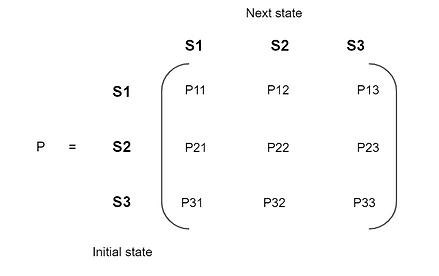
Here, Each row sums up to 1 since they are probabilities.
Markov Property: The basic property of a Markov chain is that only the most recent point in the trajectory affects what happens next. This is called the Markov Property. It means that Xt+1 depends only upon Xt, and it does not depend upon Xt−1, . . . , X1, X0.
We formulate the Markov Property in mathematical notation as follows:
P(Xt+1 = s | Xt = st , Xt−1 = st−1, . . . , X0 = s0) = P(Xt+1 = s | Xt = st),
for all t = 1, 2, 3, . . . and for all states s0, s1, . . . , st , s.

Markov chains have many applications as statistical models of real-world processes, such as studying cruise control systems in motor vehicles, queues or lines of customers arriving at an airport, currency exchange rates, and animal population dynamics.
Markov processes are the basis for general stochastic simulation methods known as Markov chain Monte Carlo, which are used for simulating sampling from complex probability distributions, and have found application in Bayesian statistics, thermodynamics, statistical mechanics, physics, chemistry, economics, finance, signal processing, information theory, and speech processing.
Let us consider one real-life example to understand how its practically applied to solve a problem.
1. Markov chains to predict stock market trends
We want to model the stock markets trend. So first recall our assumption that a stocks market movement is random.
Therefore there is a dynamic system we want to examine — the stock markets trend.
We can identify that this system transitions randomly, between a set number of states.
All possible collections of all these states are called state-space. For our case, we can identify that a stock markets movement can only take on three states (the state-space):
● Bull markets: periods of time where prices generally are rising, due to the actors having optimistic hopes of the future.
● Bear markets: periods of time where prices generally are declining, due to the actors having a pessimistic view of the future.
● Stagnant markets: periods of time where the market is characterized by neither a decline nor a rise in general prices.
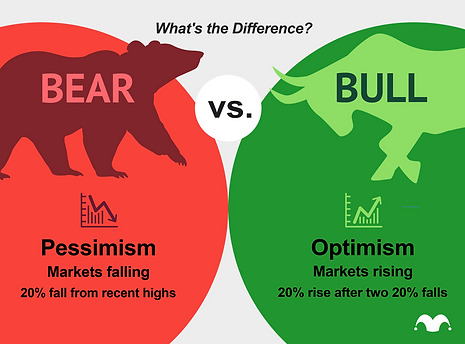
In fair markets, it is expected that the market information is distributed equally among its actors and that prices fluctuate randomly. This means that every actor has equal access to information such that no actor has an upper hand due to inside information. Through technical analysis of historical data, certain patterns can be found as well as their estimated probabilities.
After a week characterized by a bull market trend, there is a 90% chance that another bullish week will follow. Additionally, there is a 7.5% chance that the bull week instead will be followed by a bearish one or a 2.5% chance that it will be a stagnant one. After a bearish week, there’s an 80% chance that the upcoming week also will be bearish, and so on as represented in the state transition diagram below:
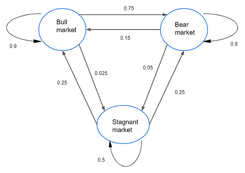
The state transition diagram
By compiling these probabilities into a table, we get the following state transition matrix M:

The transition probability matrix
We then create a 1×3 vector C which contains information about which of the three different states any current week is in; where column 1 represents a bull week, column 2 a bear week, and column 3 a stagnant week. In this example we will choose to set the current week as bearish, resulting in the vector C = [0 1 0].
Given the state of the current week, we can then calculate the possibilities of a bull, bear, or stagnant week for any number of n weeks into the future. This is done by multiplying the vector C with the matrix, giving the following:
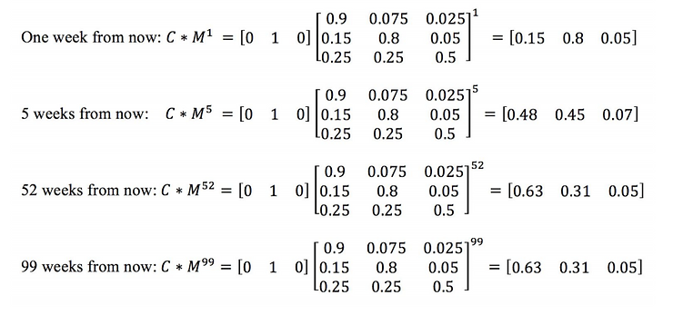
A characteristic of what is called a regular Markov chain is that, over a large enough number of iterations, all transition probabilities will converge to a value and remain unchanged. This means that, after a sufficient number of iterations, the likelihood of ending up in any given state of the chain is the same, regardless of where you start.
So, when the chain reaches this point, we can say the transition probabilities reached a steady-state.
This is what Markov ultimately wanted to prove!
From this we can conclude that as n → ∞ , the probabilities will converge to a steady-state, meaning that 63% of all weeks will be bullish, 31% bearish, and 5% Stagnant. What we also see is that the steady-state probabilities of this Markov chain do not depend upon the initial state. The results can be used in various ways, some examples are calculating the average time it takes for a bearish period to end or the risk that a bullish market turns bearish or stagnant.
2. Predict mutating virus using Markov Chain
A virus can exist in N different strains. At each generation, the virus mutates with probability α ∈ (0, 1) to another strain which is chosen at random. Very (medically) relevant question: what is the probability that it is in the same strain after n generations?

We let Xn be the strain of the virus in the nth generation, which is a random variable with
values in {α, β}. We start with X0 = α. A key point here is that the random variables Xn and
Xn+1 are not independent; we’ll come back to this later.
The probability that we are interested in is:
pn = P(Xn = α | X0 = α)
We can try to find this probability by considering what happens at time n + 1. We can have
Xn+1 = α in two ways: either (i) Xn = α and then the virus does not mutate, or (ii) Xn = β and
then the virus mutates. This leads us to the equation:
pn+1 = pn · (1 − p) + (1 − pn) · p
More carefully, what we are using here is the law of total probability with the partition {Xn =
α}, {Xn = β}:
P(Xn+1 = α) = P(Xn+1 = α | Xn = α)P(Xn = α) + P(Xn+1 = α | Xn = β)P(Xn = β).
But P(Xn+1 = α | Xn = α) = 1 − p (no mutation) and P(Xn+1 = α | Xn = β) = p (mutation),
while P(Xn = α) = pn (by definition) and P(Xn = β) = 1 − pn (complementary events).
If we were being more careful, we would explicitly include the condition X0 = α in all our
expressions. This makes the calculation look a bit more cumbersome, but becomes useful for more involved examples. Then our starting point becomes:
P(Xn+1 = α | X0 = α) = P(Xn+1 = α | Xn = α, X0 = α)P(Xn = α | X0 = α)
+ P(Xn+1 = α | Xn = β, X0 = α)P(Xn = β | X0 = α)
Now from (2.1) we obtain for the desired quantity pn the recursion relation:
pn+1 = p + (1 − 2p) · pn, (n ≥ 0),
with the initial condition p0 = 1. This has a unique solution given by
you can easily check that this works! As n → ∞ this converges to the long term probability that the virus is in strain α, which is 1/2 and therefore independent of the mutation probability p.
We return briefly to our comment about Xn+1 and Xn not being independent. We saw that
P(Xn+1 = α) = pn+1 = p + (1 − 2p)pn < 1 − p,
for n > 0, since pn < 1 for n > 0. But then, for n > 0,
P(Xn = α, Xn+1 = α) = (1 − p)P(Xn = α) > P(Xn+1 = α)P(Xn = α),
contradicting the definition of independence. Another way to express the last formula is
P(Xn+1 = α | Xn = α) > P(Xn+1 = α),
for n > 0. Indeed, as n → ∞ we know that the right-hand side here tends to 1/2, while the
left-hand side is always (1 − p) > 1/2.
The theory of Markov chains provides a systematic approach to this and similar questions.
The possible values of Xn constitute the state space S of the chain: here S = {α, β}. The characteristic feature of a Markov chain is that the past influences the future only via the present. For example
P(Xn+1 = α | Xn = α, Xn−1 = α) = P(Xn+1 = α | Xn = α).
Here the state of the virus at time n + 1 (future) does not depend on the state of the virus at time n − 1 (past) if the state at time n (present) is already known.
3. Natural Language Generation(NLG) using Markov Chain
According to Wikipedia, Natural language generation (NLG) is the natural language processing task of generating natural language from a machine representation system such as a knowledge base or a logical form. Psycholinguists prefer the term language production when such formal representations are interpreted as models for mental representations.
While there are so many different ways starting from a simple-rule-based Text Generation to using highly advanced Deep Learning Models to perform Natural Language Generation, Here we will explore a simple but effective way of doing NLG with the Markov Chain Model using Markovify python library.
Markovify is a simple, extensible Markov chain generator. Right now, its main use is for building Markov models of large corpora of text and generating random sentences from that. But, in theory, it could be used for other applications.
Installation:
!pip install nltk
!pip install spacy
!pip install markovify
!pip install -m spacy download en
We will be using NLTK and spaCy for text preprocessing since they are the most common and our model will generate text better if we parse it first. Now we can import our libraries.
import spacy
import re
import markovify
import nltk
from nltk.corpus import gutenberg
import warnings
warnings.filterwarnings('ignore')nltk.download('gutenberg')
!python -m spacy download en
For this demo, we are going to use three of Shakespeares’ Tragedies from the Project Gutenberg NLTK corpus. We will first print all the documents in the Gutenberg corpus so you can mix and match these as you please.
#inspect Gutenberg corpus
print(gutenberg.fileids())
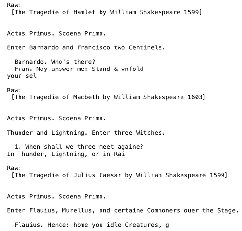
We are going to use the three Shakespeare Tragedies Macbeth, Julius Caesar, and Hamlet. So we will next import them and inspect the text.
#import novels as text objects
hamlet = gutenberg.raw('shapespeare-hamlet.txt')
macbeth = gutenberg.raw('shakespeare-macbeth.txt')
caesar = gutenberg.raw('shakespeare-caesar.txt')#print first 100 characters of each
print('nRaw:n', hamlet[:100])
print('nRaw:n', macbeth[:100])
print('nRaw:n', caesar[:100])
Next, we will build a utility function to clean our text.
#utility function for text cleaning
def text_cleaner(text):
  text = re.sub(r'--', ' ', text)
  text = re.sub('[[].*?[]]', '', text)
  text = re.sub(r'(b|s+-?|^-?)(d+|d*.d+)b','', text)
  text = ' '.join(text.split())
  return text
Next, we will continue to clean our texts by removing chapter headings and indicators and apply our text cleaning function.
#remove chapter indicator
hamlet = re.sub(r'Chapter d+', '', hamlet)
macbeth = re.sub(r'Chapter d+', '', macbeth)
caesar = re.sub(r'Chapter d+', '', caesar)#apply cleaning function to corpus
hamlet = text_cleaner(hamlet)
caesar = text_cleaner(caesar)
macbeth = text_cleaner(macbeth)
We now want to use spaCy to parse our documents. More can be found here on the text processing pipeline.
#parse cleaned novels
nlp = spacy.load('en')
hamlet_doc = nlp(hamlet)
macbeth_doc = nlp(macbeth)
caesar_doc = nlp(caesar)
Now that our texts are cleaned and processed, we can create sentences and combine our documents.
hamlet_sents = ' '.join([sent.text for sent in hamlet_doc.sents if len(sent.text) > 1])
macbeth_sents = ' '.join([sent.text for sent in macbeth_doc.sents if len(sent.text) > 1])
caesar_sents = ' '.join([sent.text for sent in caesar_doc.sents if len(sent.text) > 1])shakespeare_sents = hamlet_sents + macbeth_sents + caesar_sents#inspect our text
print(shakespeare_sents)
Our text pre-processing is done and we can start using Markovify to generate sentences.
#create text generator using markovify
generator_1 = markovify.Text(shakespeare_sents, state_size=3)
And now for the fun part. We just need to write a loop to generate as many sentences as we want. Below, we will create 3 sentences of undefined length and 3 more with a length of fewer than 100 characters.
#We will randomly generate five sentences
print("Longer sentences:")
for i in range(5):
    print(generator_1.make_sentence())

print()
print("Shorter sentences:")

#We will randomly generate three more sentences of no more than 100 characters
for i in range(5):
    print(generator_1.make_short_sentence(max_chars=100))

Not bad for Shakespearean English. But I think we can do better. We will implement POSifiedText using SpaCy to try and improve our text prediction.
class POSifiedText(markovify.Text):   def word_split(self, sentence):
      return ['::'.join((word.orth_, word.pos_)) for word in nlp(sentence)]   def word_join(self, words):
      sentence = ' '.join(word.split('::')[0] for word in words)
      return sentence#Call the class on our text
generator_2 = POSifiedText(shakespeare_sents, state_size=3)
And finally, print more sentences using our new generator.
print("Longer sentences:")
#now we will use the above generator to generate sentences
for i in range(5):
    print(generator_2.make_sentence())

print()
print("Shorter sentences:")
#print 100 characters or less sentences
for i in range(5):
    print(generator_2.make_short_sentence(max_chars=100))

Conclusion
A Markov chain is a stochastic process containing random variables transitioning from one state to another which satisfies the Markov property which states that the future state is only dependent on the present state.
We can construct a model by knowing the state-space, initial probability distribution q, and the state transition probabilities P. To know a future outcome at time n away from now, we carry out the basic matrix multiplication: q*P^n
To figure out the stationary distribution which ultimately tells us where the probabilities effectively tilt to a certain state more than others, we run several simulations to create a long series chain. The frequency of states in a series chain is proportional to its number of connections in the state transition diagram. The P matrix plays a huge role here too.
Markov chains were initially discovered as a result of proving that even dependent outcomes follow a pattern. Historically it was believed that only independent outcomes follow a distribution. As we have seen, even Markov chains eventually stabilize to produce a stationary distribution.
Nowadays Markov chains are used in everything, from weather forecasting to predicting market movements and much much more.
Thanks for reading !!!
References:
https://en.wikipedia.org/wiki/Markov_model
https://www.stat.auckland.ac.nz/~fewster/325/notes/ch8.pdf
http://personal.strath.ac.uk/x.mao/teaching/MM307/note2.pdf
Source: Auto Draft
Never Miss an Update
Get notified when we publish new analysis on HFT, market microstructure, and electronic trading infrastructure. No spam.
Subscribe by EmailHFT Systems Architect & Consultant | 20+ years architecting high-frequency trading systems. Author of "Trading Systems Performance Unleashed" (Packt, 2024). Creator of VisualHFT.
I help financial institutions architect high-frequency trading systems that are fast, stable, and profitable.
>> Learn more about what I do:
https://hftAdvisory.com
>> Your execution logs contain $200K+ in recoverable edge.
>> Microstructure Diagnostics — one-time audit, 3-5 day turnaround
https://hftadvisory.com/microstructure-diagnostics
... more info about me 👇
